8.4. Calculating Areas
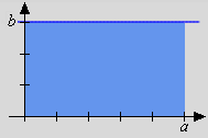
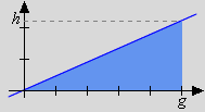
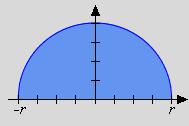
There are some integrals that allow quite an interesting interpretation. The three examples to follow are accompanied by a sketch of their integrands.
-
For we have:
|
|
-
For we have:
|
|
|
|
In each case the integral value coincides with the area of the respective object (rectangle, triangle, semi-circle) as known from elementary geometry. All of the three regions are bounded from below by the x-axis and from above by the integrand f. We understand those regions as being generated by the "boundary function" f on the interval of integration.
This coincidence between areas and integrals raises hope to calculate areas of further regions in the plane by means of integration, especially those curvilinear ones which are not covered by common geometry. The following sketch will put this hope into practice.
Take some positive, integrable function . For an arbitrary we now divide the interval into n subintervals (and advantageously rename the endpoints a and b):

As we may split integrals unrestrictedly, the mean value theorem [8.2.8] allows to calculate the integral of f as a sum
[1]
where each addend is the product of the respective subinterval's diameter with a suitable value of f. As f is positive we may interpret this product as the area of a rectangle, and the integral thus as the sum of rectangle areas.
Depicted below is the function and the region it generates on the interval . Moving the slider will approximate this region by a union of rectangles. Their heights are set according to [1] thus the sum of all rectangle areas has always the same value
13,8
i  |
|
|
i.e. the value of the integral of f.
Consider:
-
The series in [1] is a constant one, and thus trivially convergent to
. [2]
This context explaines the ideas behind the symbols and dx introduced by Leibniz: In the limit process the subintervals shrink up to only one point x, that means the actual difference transmutes into the infinitesimale difference dx, leaving only one choice for namely x, and finally the sigma sign mutates to , a stylized, elongated letter S. The limit [2] is thus symbolically noted as
With positive functions we now may understand an integral also as an area. With arbitrary functions however this won't be true as areas are always positive in contrast to integrals.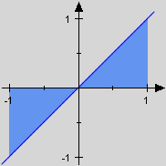 As an example the area of the region generated by the identity function X and the x-axis on calculates to 1, and is thus not replaceable by the integral . As an example the area of the region generated by the identity function X and the x-axis on calculates to 1, and is thus not replaceable by the integral .
A sheer integral coincides with an area only in suitable cases. But how to proceed then with regions generated by an arbitrary, not solely positive function?
As reflection in the x-axis is "areaproof" the solution would be to reflect all the segments of f lying underneath the x-axis leaving the others untouched. But this is actually the transition from f to .
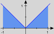 And indeed the area of the region generated by X is now exactly calculated by the integral . And indeed the area of the region generated by X is now exactly calculated by the integral .
In the following definition we confine ourselves to continuous functions f. So we don't have to worry about the integrability of and furthermore these functions meet our ideas of the kind of boundary a region in the plane should have.
|
Definition: If f is a continuous function on , i.e. , we call the number
|
[8.4.1] |
the area of the region generated by f and the x-axis on [a,b].
|
For calculating areas we thus need primitives of instead of primitives of f. But with functions that have only a finite number of zeros this additional difficulty is niftily overcome with the following 3-step-method:
-
Calculate all zeros of f in and put them, combined with and , into their natural order: .
-
Calculate all integrals of the kind .
-
As f is continuous it has a uniform sign in each of the intervals . Due to [8.2.12] we thus may interchange integration with calculating the absolute value. Now get the area by summation of the above integrals in their absolute value:
|
Example:
-
We calculate the area of the region generated by and the x-axis on :
-
. Due to the decomposition we have to consider three integrals, namely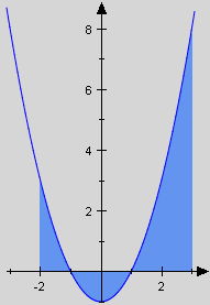
-
-
The area now amounts to .
-
Next we calculate the area of the region generated by and the x-axis on .

-
As we have to look for the odd multiples of π within which yields the decomposition , so we have to calculate only two integrals this time:
-
and
-
The resulting area therefore is .
|
All regions considered so far are bounded by the x-axis, so they have at least one straight edge.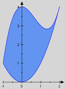 With a simple trick however we can use our methods developed so far to cope with regions that are entirely bounded by curvilinear lines. The following example will show this. With a simple trick however we can use our methods developed so far to cope with regions that are entirely bounded by curvilinear lines. The following example will show this.
The region to the left is generated by two positive functions, by the upper function

i 
|
|

|
and the lower one .

i  |
|

|
Obviously the area of the region generated by f on is too big. The excess is exactly the area of the region generated by g on . Thus the actual area is easily computed as their difference:
There is no doubt in our sketch which function is the upper one and which is the lower. More common situations may not be assorted that well, and functions that intersect more than twice could not be ordered in this way at all! But similar to the introduction of areas, problems like this are superbly solved by the absolute value:
|
Definition: For any two functions we call the number
|
[8.4.2] |
the area of the region generated by f and g on [a,b].
|
Consider:
-
Often both functions will have a lowermost and an uppermost point of intersection, say a and b. In this case we use area of the region generated by f and g as a shortened notation for .
-
When calculating the x-axis' position has actually no meaning. If parts of the region generated by f and g are lying underneath the x-axis, a vertical scrolling by an appropriate amount, perhaps c units, will yield a region lying entirely above the x-axis. Its area however calculates to:
-
The area of the region generated by f and g on [a,b] is by definition that of the region generated by and the x-axis on [a,b]. Thus the above 3-step-method is applicable.
As an example we calculate the area of the region used in our introduction, i.e. the region generated by and . To that end we only need to consider the region generated by
-
f and g intersect only twice so that we have to consider just one integral.
-
-
The area of the region generated by f and g thus amounts to .
The region generated by a positive function and the x-axis on [a,b] is in fact the set
.
Further, for each , the positive value could be regarded as the diameter of the interval . If we understand this interval as a section
in the set M we obviously get the two-dimensional area of M, i.e. the number , by integrating the one-dimensional diameters of its sections . We will elaborate this aspect in the next part and develop from that a recursive method to calculate the content of higher-dimensional solids.
|



 As an example the area of the region generated by the identity function X and the
  And indeed the area of the region generated by X is now exactly calculated by the integral .

 With a simple trick however we can use our methods developed so far to cope with regions that are entirely bounded by curvilinear lines. The following example will show this.