8.6. Calculating the Length of a Path
We now consider paths and their lengths. This will finish the geometry section in our integral course.
|
Definition: Let be a subset of . If is a closed interval in we call any function
|
[8.6.1] |
a path (in M). is the initial point and the final point of w. The path w is closed if its initial and final points coincide: . The range is called the curve belonging to w and the path [8.6.1] is then regarded as a parametrization of its curve.
If all the coordinate functions are
-
continuous then w is a continuous path (occasionally: -path).
-
differentiable, w is a differentiable path (-path) and the function
|
[8.6.2] |
is called the derivative of w. w is a regular path if for all .
Repeatedly differentiable paths and higher derivatives are introduced analogously.
-
continously differentiable, w is called a smooth path (-path).
-
integrable, then w is an integrable path and for any the vector
|
[8.6.3] |
is read as the integral of w from r to s.
|
Consider:
If is a common real-valued function, its graph is the curve belonging to the path
.
As X is arbitrary often differentiable (thus continuous and integrable as well), w has the same qualities as f has.
The path concept is, among others, designed to describe movement. In this case it is the movement of a particle along its way, with the interval being the section of time in which the movement is monitored. The notation
(instead of ) supports this perception. If w is we interpret the derivative as the speed of the particle at time t.
There is a clear difference between a path and the associated curve. A single curve may belong to several different paths. For an example consider the paths
Both of them produce the line segment between and , but they differ in their running direction: Whereas w generates the line segment from left to right, v does it the reverse way.
Also, running through a curve repeatedly will change the path but not the curve. If we substitute in the following example the interval by the ellipse will be cycled k-times. But this of course won't alter its shape.
Finally we note that cutting constant segments (i.e. for all ) will leave the curve untouched, but not the path.
|
Example:
-
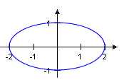 With the ellipse With the ellipse
is a closed -path in . The sketch shows the associated curve for and .
-
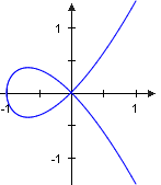 The -path The -path
is not closed and as and the curve runs through twice.
-
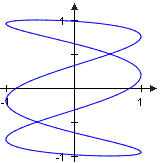 Lissajous-curves are generated by the following -paths: Lissajous-curves are generated by the following -paths:
The sketch shows the Lissajous-curve for and . Lissajou-curves are not always closed.
-
The
spiral
i   |
| left mouse: rotate | right mouse: context menu |
spiral
Display by JavaView
|
and the closed
curve of Viviani
i   |
| left mouse: rotate | right mouse: context menu |
curve of Viviani
Display by JavaView
|
are examples for -curves in .
-
The Famous Curves Index is a large collection of curves.
|
Some basic derivation rules and and a version of the mean value thoerem are valid for differentiable paths.
|
Proposition:
-
For any differential paths each linear combination is differentiable and
|
[8.6.4] |
-
If is a differentiable path then for any two different points there are numbers
between
i   |
|
i.e. , if
and , if .
|
r and s such that
|
[8.6.5] |
-
If is a differentiable path the derivative is integrable and
|
[8.6.6] |
for all .
Proof:
1. ► According to the sum and factor rule all coordinate functions are differentiable and
2. ► Let be an arbitrary coordinate function. The mean value theorem [7.9.5] provides a between r and s such that
3. ► Every coordinate function is certainly a primitive for .
|
The integral of a path satisfies the same calaculation rules and has the same properties just as a usual integral.
|
Proposition: If are integrable paths we have for all
:
-
|
[8.6.7] |
-
|
[8.6.8] |
-
If r and s are different there are numbers between r and s such that
|
[8.6.9] |
Proof: We prove the respective identity coordinatewise and succeed in
1. ► with [8.2.2] - [8.2.4].
2. ► with [8.2.5]/[8.2.7].
3. ► with [8.2.8].
|
The estimate [8.2.11] is transferable to continuous paths, an essential step in our theory. The notation and the proof as well use the common
dot product
i   |
|
The dot product
in particular provides the length of a vector . Our proof uses the simple identity
,
and the Cauchy-Schwarz inequality
Its proof and further properties of the dot product, as e.g. the triangle inequality
are to be found in part 9.13.
|
in .
|
Proposition: For any continuous path the following inequality holds:
|
[8.6.10] |
Proof: First we note that the paths w and are continuous and thus integrable. With the abbreviation
, thus
the following calculation is easier to follow. For there is nothing to prove because the right side of [8.6.10] is always positive. So we may assume . According to the Cauchy-Schwarz inequality and due to the integral monotony [8.2.10] we may estimate as follows:
|
We are now going to calculate the length of a continuous path w. The actual key concept in calculating areas then was to approximate the region in question by a sequence of elementary regions (union of rectangles) with a known area. Analogously we will now try to approximate the path w by elementary paths, namely the union of line segments.
We start with some technical preparations: A finite sequence in , , such that
is called a partition of the interval with the number being its fineness.
For a given path w any partition Z features
points of w and thus n consecutive line segments. We use them to create the traverse :
, if
|
[8.6.11] |
Each traverse is a path with initial point and final point . Traverses approximate a continuous path w in the following way:
|
Proposition: Let be a continuous path. Then there is for each such that
for all .
|
[8.6.12] |
for any partition Z with a fineness less than δ.
Proof: Take an arbitrary . As each coordinate function is continuous function on the closed interval it is actually uniformly continuous (see [6.5.5]). Thus there is a for such that
Setting we therefor have for any with :
[1]
Now let be an arbitrary partition with a fineness not exceeding δ. If , say , we thus know:
and .
Using [8.6.11], the triangle inequality and the estimate [1] we now see that
|
The length of a traverse is easily calculated by adding up the lengths of the line segments involved. Thus we set
|
[8.6.13] |
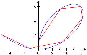 As the line segment represents the shortest distance between and we expect the length of w to be an upper bound for all . Considering [8.6.12], a sound candidate for the prospective path length would be the
supremum As the line segment represents the shortest distance between and we expect the length of w to be an upper bound for all . Considering [8.6.12], a sound candidate for the prospective path length would be the
supremum
i   |
|
We remember the completeness axiom :
In each non-empty bounded subset has a least upper bound, its supremum (termed ). An upper bound s of M equals if and only if is no upper bound of M for each .
|
of .
The depicted example on the right shows a part of one of René Descartes' Folium of Descartes, that is the path . For a three dimensional example we replenish the
spiral
i   |
| left mouse: rotate | right mouse: context menu |
spiral
Display by JavaView
|
from a former example.
|
Definition: A continuous path is a path of finite length (or a rectifiable path) if the set is bounded. In this case the number
|
[8.6.14] |
is called the length of w.
|
We will find out that smooth paths are rectifiable and, in addition, integrating the length of their derivative will provide an upper bound for all . Smoothness however is only a sufficient and not a necessary condition for a finite length, as the non-smooth path

i   |
If is a partition of we find a suitable k such that . That means:
and so we have and consequently
for all . Taking into account that
we now may estimate as follows:
|
proves.
|
Proposition: If is a smooth path then for any partition Z of the estimate
|
[8.6.15] |
holds and w is thus rectifiable.
Proof: If is an arbitrary partition we see from the properties [8.6.6], [8.6.7] and the estimate [8.6.10] that
.
|
Surprisingly, [8.6.15] could be replaced by a stronger result: The integral of is more than a common upper bound of , it is the least one and thus the length of w.
|
Proposition: For the length of a smooth path we have:
|
[8.6.16] |
Proof: Due to [8.6.15] the integral is an upper bound of . It is thus sufficient to find a partition Z for each such that
.
As the coordinate functions are continuously differentiable, each is continuous and on the closed interval even uniformly continuous. Thus there is a for such that
[2]
for all . Now take a partition with a fineness less than . According to [8.2.8] and [8.6.5] resp. we find numbers
-
such that [3]
-
such that
[4]
As we have for all i:
.
With [2] we thus know that and according to [3] and [4] we may estimate the integral of as follows (note that for any positive x, y):
This proves the required estimate . Therefor is the least upper bound of , i.e. its supremum.
|
In a former comment paths were considered as means of describing the movement of a particle. With this perception [8.6.16] just says that
the length of the path traced by the particle is the integral of its magnitude of speed .
Although [8.6.16] could replace computing a supremum (usually a difficult task) with calculating an integral, the length of a path is rarely simple to get as the integrand is always the length of a vector, which actually is the root of a sum. The following examples will demonstrate this.
|
Example:
-
The curve belonging to the smooth path
is the line segment joining the points and in . With the constant derivative the length of w straight away calculates to
which, as expected, is the distance between a and b.
-
For an arbitrary we compute the length of
thus measuring the spiral from our initial example:
From we get (note the Pythagorean theorem : )
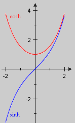
To calculate the integral we need the hyperbolic functions
sinh und cosh
i   |
 Hyperbolic sine (sinus hyperbolicus) and hyperbolic cosine (cosinus hyperbolicus) are two functions based on the exponential function exp (see [5.9.18]). For we set
[0]
sinh and cosh are arbitrary often differentiable and, as (see [7.5.8]), their derivatives are easily calculated to
and .
The following properties are also straight forward from the definition [0]:
-
-
-
-
-
-
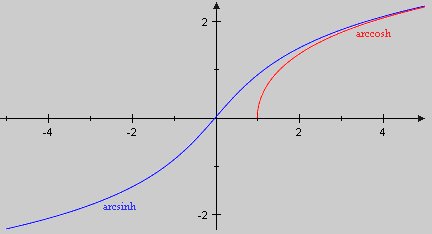
sinh is injective (according to [7.9.6] as for all x) and surjective as well (a consequence of the intermediate value theorem [6.6.2], because sinh is continuous and ). Thus sinh is bijective and its inverse function
is called arcussinus hyberbolicus. In a similar way arcuscosinus hyperbolicus is introduced, the inverse function of :
|
. As is a primitive of

i   |
|
We use the fundamental theorem [8.2.13] and employ integration by parts (see [8.3.1]) to compute for any x the integral
is thus a primitive of .
|
the integral now could be solved with the substitution formula (see [8.3.5]). We substitute and thus get
-
Surprisingly we can't find a single term that calculates the length of the ellipse given by
The integral
is a so called elliptical integral that could only be solved in the trivial cases and . In the latter however, i.e. , the ellipse is circle with radius . Its circumference thus is
.
Exercise:
-
For we have and thus
-
For the parabola segment we have . Thus
and as is a primitive of we eventually get
|
The length of smooth path would be easy to calculate if the derivative was a vector of constant length. For we even have
for all , i.e. the section of the path is as long as the section of the respective interval. In that case we say that w is parameterized by the arc length. Regular paths are always parameterizable in this way:
|
Proposition: If is a regular path then there is a -bijection such that
-
is parameterized by the arc length.
-
and w generate the same curve.
-
.
|
[8.6.17] |
Proof: Due to the fundamental theorem [8.2.13] the function given by
is a prinitive of . As w is regular we have: for all . From [7.9.6] we thus know that s is injective and that is differentiable (see [7.5.4]) at each with
Further, the intermediate value theorem [6.6.2] guarantees that because and . Now due to the chain rule [7.7.8] the path is regular and
Finally we show:
1. ►
2. ► As is bijective we see that:
3. ►
|
|
 |
|
 With the ellipse
 The -path
 As the line segment represents the shortest distance between and we expect the length of w to be an upper bound for all . Considering