7.9. The Mean Value Theorem

Extreme points are a basic concept in applied mathematics. Examples in 7.11 will demonstrate this. So we start this chapter introducing this notation.

The major part however is up to the mean value theorem and its implications. The theorem itself is easily depicted (look at the sketch in [7.9.4]), but its proof is far from being trivial. The actual clue is the extreme value theorem ([6.6.5]) for continuous functions.

The mean value theorem proves to be the most powerful device in calculus.

To illustrate this new concept we look at the function  ${\displaystyle f:[-\mathrm{2,}\infty [\to ℝ}$given by ${\displaystyle f(x)=\frac{1}{4}{x}^4-\frac{5}{6}{x}^3-\frac{1}{2}{x}^2+\frac{5}{2}x}$. The sketch to the right obviously shows that  f has a local minimum at −1 and at 2.5. The local minimum at −1 is even a global one. a local maximum at −2 and at 1. no global maximum as  f is unbounded from above.

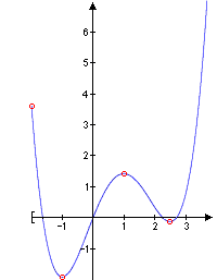Note that with the differentiable function  f a horizontal tangent is attached to all of the interior extreme points, but not to −2.

Consider:

• The ability to have an extremum is not bound to differentiability. The absolute value function ${\displaystyle |\mathrm{X}|}$ for instance has a global minimum at 0, but fails to be differentiable.

• Each global extreme point is a local one as well, because if an estimate holds for the whole of A it will certainly hold for every subset of the type ${\displaystyle A_{a,\epsilon }}$, thus for instance for ${\displaystyle A_{a\mathrm{,1}}}$. The sketch above shows that the reverse does not hold.

• As we used the relations ${\displaystyle \le }$ and ${\displaystyle \ge }$ when stating [7.9.1] a constant function has a global maximum and a global minimum at each point simultaneously. This cannot happen however when strict extrema are involved.
   

It will be an important task to detect local extreme points. As noticed above, points with horizontal tangents will play a certain role in this quest and in fact this observation leads to a first existance criterion for local extreme points.

Consider:

• The necessary criterion confirms the presumed behavior: Tangents attached to interior local extreme points are always horizontal.

• The reverse of [7.9.2] is not true (read: [7.9.2] is not sufficient). The function ${\displaystyle {\mathrm{X}}^3}$ for instance has no local extremum at 0 irrespective of ${\displaystyle ({\mathrm{X}}^3{)}^{\prime }(0)=0}$. Actually the necessary criterion only filters out points with horizontal tangents.

  Looking for suitable sufficient criteria is thus worthwhile. [7.9.17] at the end of this part is a first example for such a criterion.

• The necessary criterion is not valid at boundary points: The restriction ${\displaystyle \mathrm{X}|{ℝ}^{\ge 0}}$ has a local (even global) minimum at 0, but its derivative number at 0 is 1.

• [7.9.2] is often read as " ${\displaystyle f^{\prime }(a)=0}$ is a necessary existence condition for interior local extreme points". Thus only the first derivative's zeros come into question when searching for local extreme points.
   

Consider:

• Rolle's theorem is a pure existance theorem. It does not provide any information on uniqueness and on the precise location of ${\displaystyle \tilde{x}}$.

• The continuity at a and at b is compulsory. As an example take the function  ${\displaystyle f:[\mathrm{0,1}]\to ℝ}$ defined by  ${\displaystyle f(x)≔\{\begin{array}{l}x\text{, if }x\ne 1\hfill \\ 0\text{, if }x=1\hfill \end{array}}$. We have  ${\displaystyle f^{\prime }(x)=1}$ for all ${\displaystyle x\in ]\mathrm{0,1}[}$, although  ${\displaystyle f(0)=f(1)}$.
  But  f is discontinuous at 1.

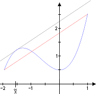
• As  ${\displaystyle f(a)=f(b)}$, the line segment joining ${\displaystyle (a,f(a))}$ and ${\displaystyle (b,f(b))}$ is horizontal. Thus Rolle's theorem is often stated in a more geometrical manner: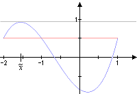

  There is an interior point ${\displaystyle \tilde{x}}$ with a tangent parallel to the line segment which joins the end point of f.

  The sketch to the right illustrates this for the function ${\displaystyle \frac{2}{3}{\mathrm{X}}^3+\frac{4}{3}{\mathrm{X}}^2-\frac{2}{3}\mathrm{X}-\frac{5}{6}}$ on the interval ${\displaystyle [-\mathrm{2,1}]}$. Apart from the marked position ${\displaystyle \tilde{x}=\frac{-2-\sqrt{7}}{3}\approx -1.55}$ there is obviously another option in this case for a horizontal tangent, namely at ${\displaystyle \frac{-2+\sqrt{7}}{3}\approx 0.22}$.
   

It is tempting to ask if this geometric property is still valid if the restriction  ${\displaystyle f(a)=f(b)}$ is lifted. The function ${\displaystyle \frac{2}{3}{\mathrm{X}}^3+\frac{4}{3}{\mathrm{X}}^2+\frac{1}{2}}$ on ${\displaystyle [-\mathrm{2,1}]}$ depicted below suggests that the answer might be "yes". Luckily we are able to prove that "yes" is the actual answer.

Theorem (mean value theorem):  There is an ${\displaystyle \tilde{x}\in ]a,b[}$ for each  ${\displaystyle f\in {\mathcal{C}}^0([a,b])\cap {\mathcal{D}}^1(]a,b[)}$ such that ${\displaystyle f^{\prime }(\tilde{x})=\frac{f(b)-f(a)}{b-a}}$ [7.9.4] Proof: We apply Rolle's theorem [7.9.3] to a modification of  f. The function

${\displaystyle g≔f-\frac{f(b)-f(a)}{b-a}(\mathrm{X}-a)}$ is certainly continuous on ${\displaystyle [a,b]}$ and differentiable on ${\displaystyle ]a,b[}$. As ${\displaystyle g(b)=f(b)-\frac{f(b)-f(a)}{b-a}(b-a)=f(a)=g(a)}$ the special condition of Rolle's theorem is met, so that due to [7.9.3] there is an ${\displaystyle \tilde{x}\in ]a,b[}$ such that ${\displaystyle 0=g^{\prime }(\tilde{x})=f^{\prime }(\tilde{x})-\frac{f(b)-f(a)}{b-a}}$. This however is the assertion.

Consider:

• On the one hand the mean value theorem is clearly an implication of Rolle's theorem due to the structure of its proof. We find on the other hand that Rolle's theorem comes as a special case from the mean value theorem, because if, in addition,  ${\displaystyle f(a)=f(b)}$ we get  ${\displaystyle f(\tilde{x})=\frac{f(b)-f(a)}{b-a}=0}$. Both theorems are thus equivalent:

  Rolle's theorem${\displaystyle \iff }$mean value theorem
  
   

With the mean value theorem one of the major results in calculus is now at our disposal. There are a lot of non-trivial applications supporting this rating. Our present notation [7.9.4] however seldom proves to be suitable for a direct application. We will thus benefit from another, equivalent version which is more taylored to application purposes. As

[7.9.4] is always valid, wheather or not a is actually left of b. Thus we will subsequently use the phrase "${\displaystyle \tilde{x}}$ lies in between a and b" as an abbreviation for

Solving [7.9.4] for  ${\displaystyle f(b)}$ provides a new version of the mean value theorem:

Let I be an arbitrary interval

i

We understand this as a common notation for open and closed intervals. In the open case we also allow the values ${\displaystyle \infty }$ for the right and ${\displaystyle -\infty }$ for the left boundery. Thus ${\displaystyle ℝ}$ and e.g. ${\displaystyle {ℝ}^{>0}}$ are regarded as intervals as well.

and let ${\displaystyle a,b\in I}$ be any two different points of I. If  ${\displaystyle f\in {\mathcal{D}}^1(I)}$, then there is an ${\displaystyle \tilde{x}}$ in between a and b such that

Consider:

• The closed interval generated by a and b is a subset of I. Any function differentiable on I is as well differentiable, and thus also continuous, on that closed subinterval. The conditions of [7.9.4] are thus satisfied.

• [7.9.5] extends (on intervals) the basic representation theorem [7.5.1] as all the values ${\displaystyle r(x)}$ now prove to be derivative numbers of  f.

• The mean value theorem is only valid for intervals. The Heaviside step function H

  i

  ${\displaystyle \mathrm{H}(x)=\{\begin{array}{l}1\text{, if }x\ge 0\hfill \\ 0\text{, if }x<0\hfill \end{array}}$

  for example is ${\displaystyle {\mathcal{D}}^1}$ on ${\displaystyle {ℝ}^{\ne 0}}$. But as ${\displaystyle {\mathrm{H}}^{\prime }(x)=0}$ for all ${\displaystyle x\ne 0}$ there will be no ${\displaystyle \tilde{x}}$ such that

  ${\displaystyle \mathrm{H}(-1)=\mathrm{H}(1)+(-1-1)\cdot {\mathrm{H}}^{\prime }(\tilde{x})}$,

  because that would imply:  ${\displaystyle 0=1}$.
   

Our first application goes back to a promise made in the context of [7.5.3/4]. Now we are able to show that regular functions on intervals are always injective.

The way the mean value theorem is used in the subsequent proof is a characteristic one: The equation [7.9.5] allows to access properties of  f as soon as global features of its derivative are available. In this case for example we know that the derivative values  ${\displaystyle f^{\prime }(x)}$ are non-zero everywhere and thus certainly non-zero as well at the normally unknown point ${\displaystyle \tilde{x}}$ provided by the mean value theorem.

A second example will classify the constant functions using only their derivative behaviour.

An appropriate statement for polynomials extends [7.9.7] considerably.

[7.9.8] allows to spot the polynomials within the ${\displaystyle {\mathcal{C}}^{\infty }}$-functions on ${\displaystyle ℝ}$ simply by checking if the zero function is one of their derivatives. The derivatives calculated in [7.8.11-13] thus prove that exp, sin and cos are no polynomials.

When dealing with continuity we introduced one of its special forms in [6.5.6], the so called lipschitz-continuity. From the mean value theorem we now get the information that a differentiable function with a bounded derivative will be lipschitz-continuous automatically.

Consider:

• Every function  ${\displaystyle f\in {\mathcal{C}}^1([a,b])}$ is lipschitz-continuous, because now  ${\displaystyle f^{\prime }}$ is a continuous function on a closed interval and thus bounded due to [6.6.4].

• As sin and cos have only values between −1 and 1, we get for all ${\displaystyle x,y\in ℝ}$:

  ${\displaystyle \begin{array}{l}|\sin x-\sin y|\le |x-y|\hfill \\ |\cos x-\cos y|\le |x-y|\hfill \end{array}}$
  
   

We are now going to extend the mean value theorem. Two options are at our disposal: We could try to find a version for two functions, as we did successfully with the intermediate value theorem (see [6.6.3]), and we could check if the mean value theorem reveals additional features if repeatedly differentiable functions are involved.

Consider:

• If we interchange a and b in [7.8.10], i.e. if we multiply the equation by −1, [7.8.10] is still valid. The second mean value theorem thus does also not depend on wheather or not a is actually left of b.
   

With the second mean value theorem we will get L'Hôpital's rule, a very efficient technique for calculating certain limits. We start with the following observation:

Let  ${\displaystyle f,g:A\to ℝ}$ be differentiable at a and assume ${\displaystyle g^{\prime }(a)\ne 0}$. If  ${\displaystyle f(a)=g(a)=0}$ then ${\displaystyle \frac{f}{g}}$ is continuously continuable at a by the limit

Proof:  At first we consider the representation (see [7.5.1] for details)

to show that a is an accumulation point

i

According to [6.4.4] we would manage this by creating a sequence ${\displaystyle (}$ in ${\displaystyle \{}$ such that ${\displaystyle a_n}$. As a is already an accumulation point of A (otherwise there would be no function differentiable at a) it is sufficient to that end to find a relative ε-neighbourhood ${\displaystyle A_{a,\epsilon }}$ satisfying ${\displaystyle A_{a,\epsilon }}$.

of ${\displaystyle \{x\in A|g(x)\ne 0\}}$. As r is continuous at a the information ${\displaystyle r(a)=g^{\prime }(a)\ne 0}$ yields a relative ε-neighbourhood ${\displaystyle A_{a,\epsilon }}$ such that ${\displaystyle g(x)\ne 0}$ for all ${\displaystyle x\in A_{a,\epsilon }\backslash \{a\}}$.

As ${\displaystyle f^{\prime }(a)=\underset{x\to a}{\lim }\frac{f(x)-f(a)}{x-a}}$ and ${\displaystyle g^{\prime }(a)=\underset{x\to a}{\lim }\frac{g(x)-g(a)}{x-a}}$  [7.9.11] now follows immediately with [6.9.8] from the equation

which holds for all ${\displaystyle x\in A_{a,\epsilon }\backslash \{a\}}$.

Consider:

• Of course are we allowed to iterate the above rules: Take e.g.  ${\displaystyle f,g\in {\mathcal{C}}^1(I)\cap {\mathcal{D}}^2(I\backslash \{a\})}$ such that  ${\displaystyle f(a)=g(a)=0}$,  ${\displaystyle f^{\prime }(a)=g^{\prime }(a)=0}$ and ${\displaystyle g^{\prime }(x),{g^{\prime }}^{\prime }(x)\ne 0}$ for all ${\displaystyle x\in I\backslash \left\{a\right\}}$.

  If the limit ${\displaystyle \underset{x\to a}{\lim }\frac{{f^{\prime }}^{\prime }(x)}{{g^{\prime }}^{\prime }(x)}}$ exists the following ones exist as well and are all the same:

  ${\displaystyle \underset{x\to a}{\lim }\frac{f(x)}{g(x)}=\underset{x\to a}{\lim }\frac{f^{\prime }(x)}{g^{\prime }(x)}=\underset{x\to a}{\lim }\frac{{f^{\prime }}^{\prime }(x)}{{g^{\prime }}^{\prime }(x)}}$.
  
   

We now turn to the second promised extension of the mean value theorem. This will, amongst others, result in a special method (Taylor polynomials) to study analytical functions.

Consider:

• If ${\displaystyle n=0}$  [7.9.16] and [7.9.5] coincide. Thus Taylor's theorem is indeed an extension of the mean value theorem.

• And again we find that the actual order of a and b is of no relevance for the validity of Taylor's theorem. The proof however is a bit more tricky this time. We need to introduce the linear function

  ${\displaystyle g≔b+(a-\mathrm{X})}$

  and to apply Taylor's formula to the composit  ${\displaystyle f\circ g}$. Noting that ${\displaystyle {(f\circ g)}^{(i)}(x)=f^{(i)}(g(x))\cdot {(-1)}^i}$, especially  ${\displaystyle f\circ g(b)=f(a)}$ and ${\displaystyle {(f\circ g)}^{(i)}(a)=f^{(i)}(b)\cdot {(-1)}^i}$, we get

  ${\displaystyle \begin{array}{ll}f(a)\hfill & =\sum _{i=0}^n\frac{f^{(i)}(b)\cdot {(-1)}^i}{i!}{(b-a)}^i+\frac{f^{(n+1)}(g(\tilde{x}))\cdot {(-1)}^{n+1}}{(n+1)!}{(b-a)}^{n+1}\hfill \\ \hfill & =\sum _{i=0}^n\frac{f^{(i)}(b)}{i!}{(a-b)}^i+\frac{f^{(n+1)}(g(\tilde{x}))}{(n+1)!}{(a-b)}^{n+1}\hfill \end{array}}$

  Thus Taylor's formula holds for  ${\displaystyle f(a)}$ as well when we take ${\displaystyle g(\tilde{x})}$ as the "new" ${\displaystyle \tilde{x}}$. So we may restate Taylor's theorem the following way:

  For any function  ${\displaystyle f\in {\mathcal{D}}^{n+1}(I)}$ and any two different points ${\displaystyle a,b\in I}$ there is an ${\displaystyle \tilde{x}}$ in between a und b that satisfies [7.9.16].

• If  ${\displaystyle f\in {\mathcal{D}}^{n+1}(I)}$ and ${\displaystyle a\in I}$ we call the polynomial

  ${\displaystyle T_{a,n}≔\sum _{i=0}^n\frac{f^{(i)}(a)}{i!}{(\mathrm{X}-a)}^i}$

  the n-th Taylor polynomial and the function ${\displaystyle R_{a,n}:I\to ℝ}$ defined by

  ${\displaystyle R_{a,n}(x)≔\{\begin{array}{l}\frac{f^{(n+1)}(\tilde{x})}{(n+1)!}{(x-a)}^{n+1}\text{, if }x\ne a\hfill \\ 0\text{, if }x=a\hfill \end{array}}$

  the n-th remainder of  f with respect to a. The function ${\displaystyle R_{a,n}}$ is well defined: There might be several ${\displaystyle \tilde{x}}$ for a fixed x satisfiying Taylor's formula, but the value  ${\displaystyle f^{(n+1)}(\tilde{x})}$ is the unique solution c of [2] belonging to x and a. ${\displaystyle R_{a,n}}$ is sometimes referred to as the Lagrange form of the remainder.

• If  ${\displaystyle f\in {\mathcal{C}}^{\infty }(I)}$ and ${\displaystyle a\in I}$ we call the power series ${\displaystyle (\sum _{i=0}^n\frac{f^{(i)}(a)}{i!}{(\mathrm{X}-a)}^i)}$ the Taylor series of  f with respect to a. If the Taylor series is convergent with r as its radius of convergence and if  ${\displaystyle f|I_{a,r}}$ is its limit function, i.e.

  ${\displaystyle f(x)=\sum _{i=0}^{\infty }\frac{f^{(i)}(a)}{i!}{(x-a)}^i}$  for all ${\displaystyle x\in ]a-r,a+r[\cap I}$,[4]

  the equation [4] is said to be the Taylor expansion of  f at a. ${\displaystyle C^{\infty }}$-functions, which allow a Taylor expansion for each ${\displaystyle a\in I}$ are thus analytical.
   

In chapter 8.10 we will access the Taylor formula in a different way. On this occasion we will learn how to test if a ${\displaystyle {\mathcal{C}}^{\infty }}$-function is analytical.

We return to the quest for local extreme points. With Taylor's formula we are now able to state a first sufficient existence criterion for local extreme points that in many cases successfully tells apart the candidates provided by the necessary criterion [7.9.2]. It is however confined to high quality functions on intervals only. Criteria for weaker functions will follow in the next part.

Consider:

• If  f is a ${\displaystyle {\mathcal{C}}^2}$-function [7.9.17] turns into the "classical" criterion
   

  ${\displaystyle f^{\prime }(a)=0\wedge {f^{\prime }}^{\prime }(a)\ne 0\Rightarrow }$f has a local extremum at a.

• The proof of [7.9.17] shows that 2. is also valid for boundary points of I. A similar result for 1. however does not hold as is demonstrated by the restriction ${\displaystyle \mathrm{X}|{ℝ}^{\ge 0}}$.

• The reverse of 2. is not true, the criterion thus not necessary. The function  ${\displaystyle f:ℝ\to ℝ}$ defined by

  ${\displaystyle f(x)≔\{\begin{array}{l}{e}^{-\frac{1}{x}}\text{, if }x>0\hfill \\ 0\text{, if }\le 0\hfill \end{array}}$

  is our counter example in this case. In 9.12 we will prove that  f is a ${\displaystyle {\mathcal{C}}^{\infty }}$-function with all its derivatives vanishing at 0 which is a local minimum point for  f.

7.8.

7.10.